## this is a comment7 Basic R
This chapter will introduce you to the basics of working with base R. After completing these exercises, you should be able to:
- Create a .Rmd and save it to your GEOG215 folder
- Use basic text and chunk formatting to create a readable knitted .Rmd file (.html)
- Read in data using a relative file path
- Execute the basics of base R by creating comments, assigning objects, and using base R functions
7.1 Creating a .Rmd and Reading Data
To follow along with this tutorial, you should create a new .Rmd document and save it into your GEOG215 folder. Every time you see code below, you should copy it to your own document!
Remove all the code chunks except for the setup chunk. You should review the formatting guidance here
7.2 Basic R Commands
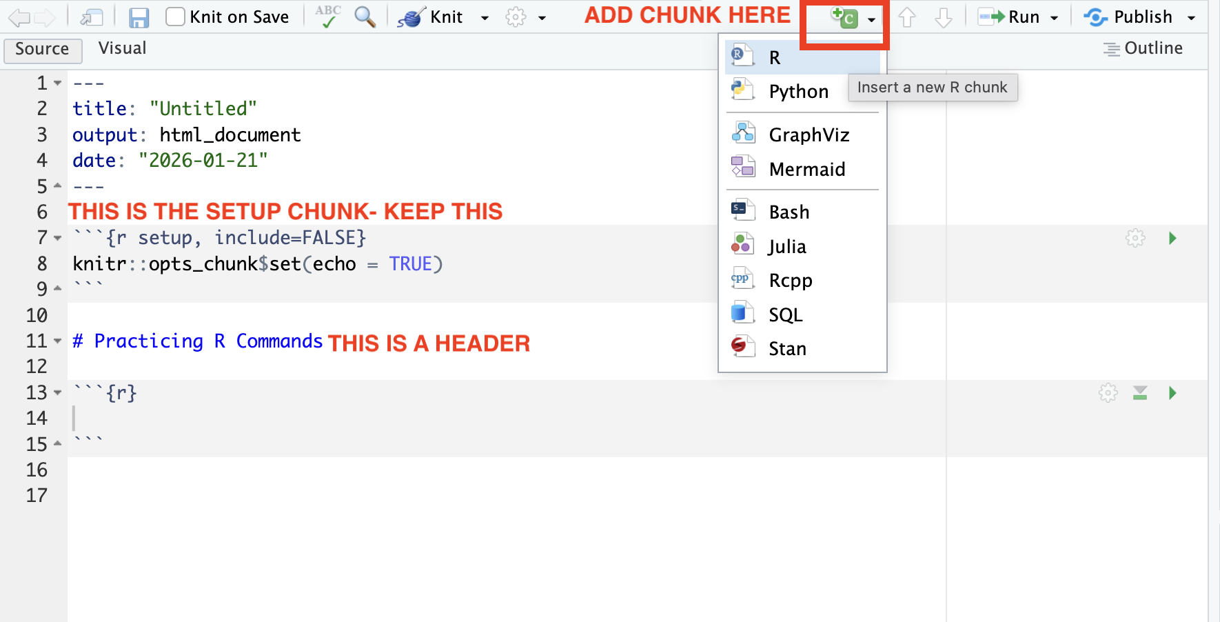
Add a new first level header called “Practicing Basic R Commands”. Then add a R code chunk below that. Your document should look like this now.
7.2.1 Making Comments
Any time you write a command, you will want to include a descriptive comment above it. To make a comment, we use this formatting.
7.2.2 Basic Math
Add the following commands to your code chunk. In addition to running a full chunk (by pressing the green arrow at the top of the chunk), you can also run a single line of code by clicking “Command” and “Return” on a Mac or “Control” and “Enter” on a PC. Run each of the following commands.
## basic addition
4 + 3

## basic division
123.1 / 3.445

##exponents
5^2
Q1: Where is the output printed when you run those commands?
Q2: Write a command that multiplies 5 by 2
7.2.3 Boolean Operators
Boolean logical operators return either a true or a false based on the conditions. Add these commands to your code chunk and run each one.
## is greater?
2 > 5

## is equal?
3 == 3

## is greater or equal?
10000 >= 1

## is less?
(3 * 5) < 20
Q3: Write a command that adds 10+7 and checks whether that is greater than 20.
7.2.4 Functions
Functions can be though of as “actions”. Base R already has many built in functions. The basic setup of a function is function(argument, ...). Add these commands to your code chunk and run each one.
#sum
sum(2:963)

#sum
mean(c(1, 10, 100, NA))

#sum, remove na
mean(c(1, 10, 100, NA), na.rm = TRUE)
Q4: Write a command that calculates the max of the following values (1, 92, 57, 12).
7.3 Assigning and Printing Objects
So far, every command we’ve run has been evaluated in the console, which means R immediately prints the result at the bottom of the chunk. This happens any time you type an expression without saving it as an object.
Saving as an object means that the result of that command is stored in our environment (look to the right, you can also double click on the object). To create objects, we use the <- command. To see the output in the console, you need to print the object. The benefit of using objects is that we can “call” that object in later commands without having to rewrite the whole command over again. Add these commands to your code chunk and run each one.
## save an object
math_object <- 4 + 3

## print an object
math_object
Q5: Create an object called my_first_object and assign the string “Hello World” to it. Then print the object.
7.4 Data Types
R works with several fundamental data types. Remember that the data type has to do with the data values:
- Numeric: numbers with decimals
- Integer: whole numbers
- Character: text data (strings)
- Logical: True/False values
- Factor: Categorical data with predefined levels
- NA: Missing data
You can check the data type using the class() command. Add these objects to your code chunk. Then write a command to check the data type of each object.
x <- 5

y <- 10L #R stores numbers as numeric, unless you specify

text <- "North Carolina" #Try running this without the quotations

sample <- "10" #try adding sample to x. What happens? Why?

logical <- 3 > 1

rural <- factor(c("Urban", "Rural"))
Q6: What happens if you values are not the expected data type? For instance, if you wanted to add sample to x?
7.5 Data Structures
R organizes data into several common structures. These structures determine how values are stored and how you can work with them. Remember that data structure has to do with how values (of any type) are stored
- Vector: Collection of items that are all the same data type
- List: Collection of items that can be different data types
- Matrix: Two-dimensional table of values, all of the same data type
- Data Frame: Two-dimensional table where columns can be different data types
You can check the structure of any object using the str() command. Add the following objects to your chunk and check the structure of each:
v <- c(1, 5, 10, 20) #note that c() is used to combine

l <- list(1, "NC", TRUE)

m <- matrix(1:6, nrow = 2)

df <- data.frame(a = 1:3, b = c("x", "y", "z"))
7.6 Adding Text and Knitting Practice
Below the code chunk, you can write in regular text. This is the benefit of using .Rmd documents– you can seamlessly integrate both code and text. Below your “Practicing Basic R Commands” chunk, add some text that describes the main things you learned in that section.
Then “Knit” your document using the “Knit” button on the top panel. Knitting creates a .html version of your .Rmd. It will open in a new tab.
7.7 Reading in a File
Below your “Practicing Basic R Commands” chunk, add a new first-level header called “Reading in and Manipulating Data”.
Download this file into your GEOG215 folder. Then use a “relative file path” to read in the data using this command:
nc_example <- read.csv("RELATIVEFILEPATH")7.8 Indexing and Subsetting
Indexing is used to select or subset elements from data structures.
[]selects elements by position[[]]extracts a single element$extracts a column by name- Logical indexing selects elements that meet a condition
Add these commands to your chunk. Run each command and add a comment based on what the command is doing.
#
nc_example[1, ]

#
nc_example[, 2]

#
nc_example[3, 1]

#
nc_example[2:4, 3]

#
nc_example$population

#
nc_example[["population"]]

#
nc_example[nc_example$population > 300000, ]


#
nc_example[nc_example$has_university == "Yes", ]
7.9 Creating a New Variable
We can create new variables using the $ command. Add this command and a descriptive comment
#
nc_example$pct_urban = 1 - nc_example$pct_rural
7.10 Mini-Challenge
Add a new first level header called “Mini-Challenge #1”. Under that header, add a code chunk. In the code chunk, write commands to do the following:
- Add a variable to the nc_example data frame called “pop_million” that calculates the population of each county in millions
- Using the nc_example data frame, create a new object called triangle_region that contains only the counties located in the Piedmont region.
- Extract the pct_rural value for Orange County
- Using the triangle-region object you created, calculate and print the mean population of the Triangle counties
- Create a new object called very_rural that returns a filtered data frame containing only counties where more than 20% of the population is rural