install.packages("tmap")
install.packages("maptiles")
install.packages("tidyverse")
install.packages("gt")
install.packages("sf")
install.packages("sp")
install.packages("spdep")
install.packages("sfdep")
install.packages("terra")
install.packages("e1071")
install.packages("car")
install.packages("spatstat")
install.packages("gstat")
install.packages("stars")
install.packages("spatialreg")
install.packages("tigris")
install.packages("deldir")6 Working in R and R Studio
This is NOT a coding class, but we will be using R for our data analysis. Because of this, while I don’t expect you to be able to generate code independently, I do expect you to develop a competency in navigating the RStudio environment and modifying code that I give you to complete specific tasks. This chapter will introduce you to R and RStudio.
RStudio is an Integrated Development Environment (IDE) for R. RStudio provides a user-friendly interface for working with R code. R is an open-source programming language that has excellent capabilities for analyzing and visualizing spatial data.
6.1 Downloading and Installing R and RStudio
To use R and RStudio, you will need to download and install both programs on your computer.
Download R (make sure to download the correct version for your operating system)
Once you have downloaded and installed RStudio, open up the application. We need to change one global setting before we start. You only need to do this once! Navigate Tools > Global Options, unclick “Restore .RData into Workspace at Startup” and choosing Never on the “Save workspace to .RData on exit”.
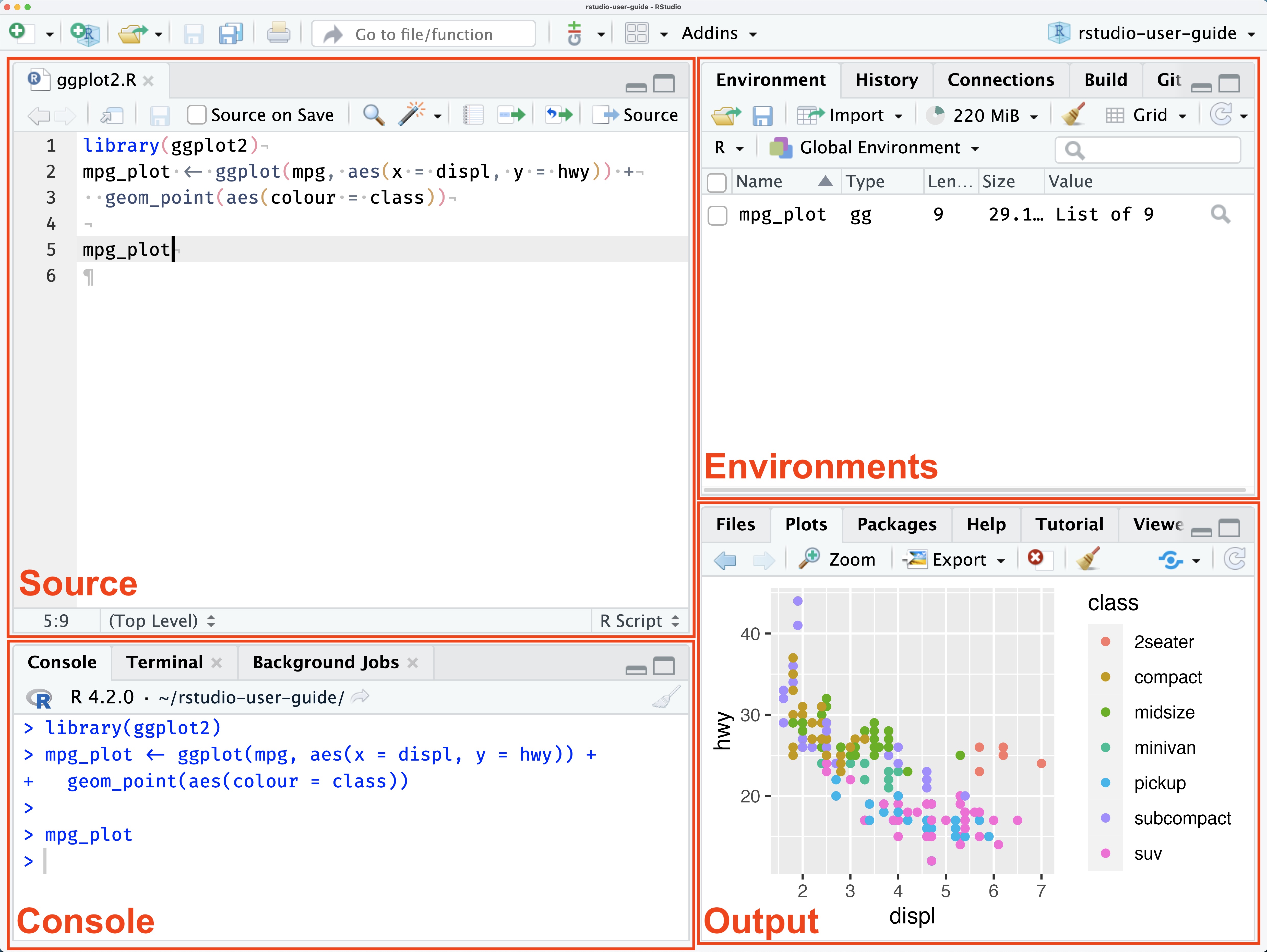
6.2 The RStudio Environment
The RStudio environment consists of four panels.
- Source: This is where you can edit R files (either .R or .Rmd) and run R code.
- Console: The console is an interactive R environment, where you can easily run R commands. Commands written in the console are not saved into any file. It can be good to use the console for quickly testing R code
- Environment: This is where R objects made during each session will appear.
- Output: This is where charts and graphs will appear.
6.3 Creating and Saving Files
In this class, we will primarily be working with .Rmd files. An R Markdown or .Rmd is a document format that is designed to easily integrate text and code. This means that you can easily type answers to questions, descriptions of code outputs, and other assignment tasks within the same document as your code.
To make a new .Rmd file, navigate to File > New Script > R Markdown
I will sometimes provide you a .Rmd template for in-class exercises. You should save these files into a GEOG391 folder on your computer (not in the downloads folder please!)
6.4 Downloading Packages
R packages extend the functionality of Base R and must be downloaded. We will use a small set of libraries in this class.
- tmap: This is the main mapping package we will use
- maptiles: This package helps us add basemaps to our maps
- gt: We will use this package to create nice tables
- tidyverse: This is the package we will use to create “tidy” analysis workflows. Tidyverse also includes ggplot2 which will be our main package to create graphics
- sf: This package allows us to read and manipulate spatial datasets
- sp: Another package for manipulating spatial data
- terra: This package allows us to read and manipulate rasters
- spdep: We use this package to create neighborhood definitions for spatial data
- sfdep: Allows the spdep package to interact with sf package
- car: Includes basic statistical functions
- e1071:Includes basic statistical functions
- spatstat:Includes spatial statistical functions
- gstat: Geostatistical modeling
- stars: Spatial statistical modeling
- spatialreg: We will use this package to run spatial regressions
- tigris: This package helps us get geographic boundaries
- deldir: Calculates Voronoi tessellation
You should copy and paste each of these commands into the Console one by one to download the packages.
Once you have downloaded the packages, you will need to load them every time you want to use them. I will always tell you what packages to load!
Download your first .Rmd template for this class (very exciting)! Save this file into your GEOG391 folder.
6.5 Basic .Rmd Functionality
Welcome to your first .Rmd! Each .Rmd starts with a header, where you can change the name and the date. Change the header to your name and the current date
A .Rmd is made up of two main components: code chunks (this is where you write code) and text (any words that are outside of a code chunk). Any time you are writing code, it needs to be in a code chunk. Chunks can then be run to execute the code within the chunk. The idea of chunking is to group code that accomplishes a single, related task into one code chunk. When you begin a new step or process in your workflow, you start a new chunk.
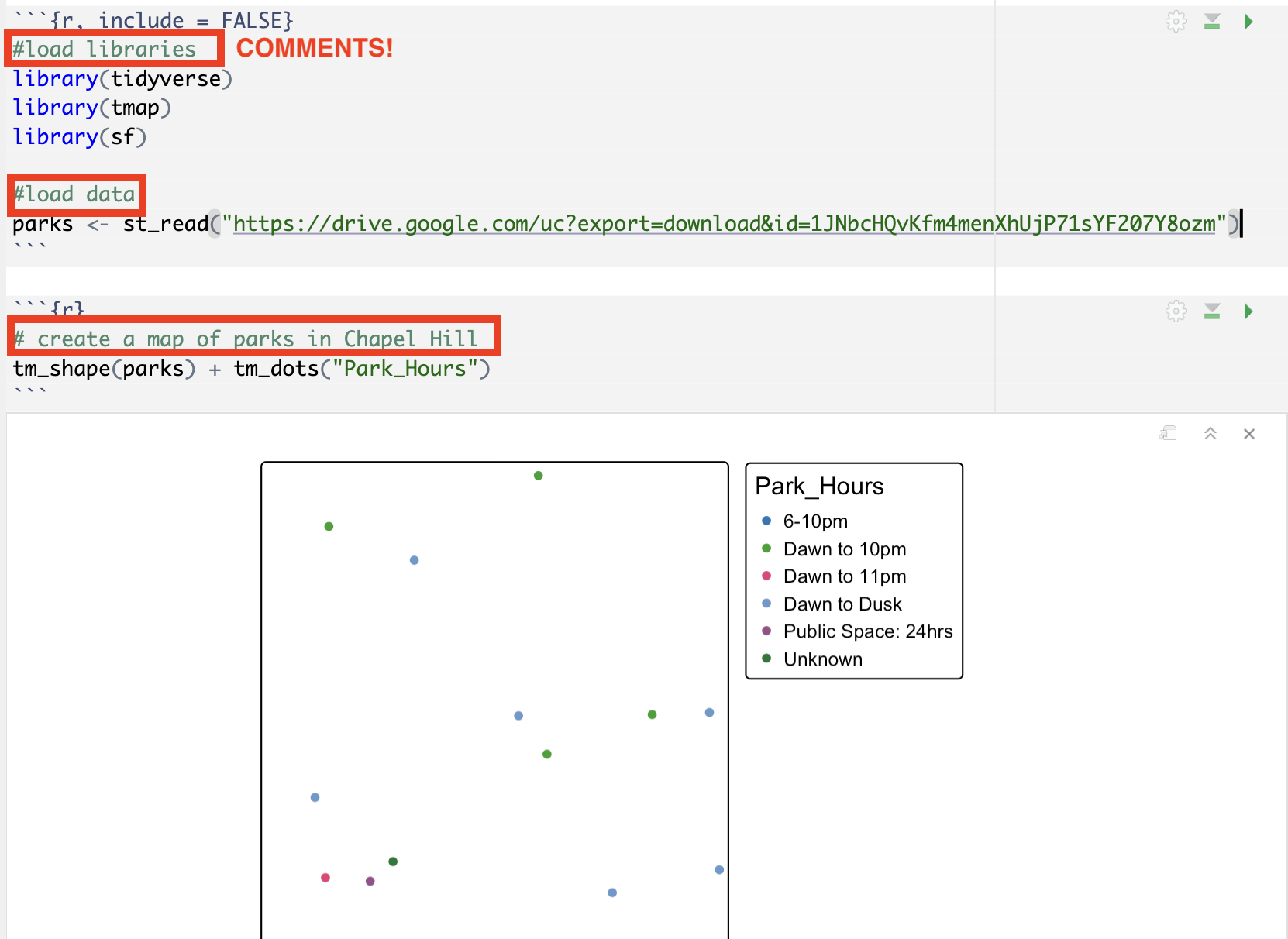
Your .Rmd template already has a header (where you can change the name and date) and two code chunks. The first code chunk is the SET UP CHUNK. The second code chunk is the LIBRARY AND DATA CHUNK. To load the libraries and data, you should RUN CODE CHUNK.

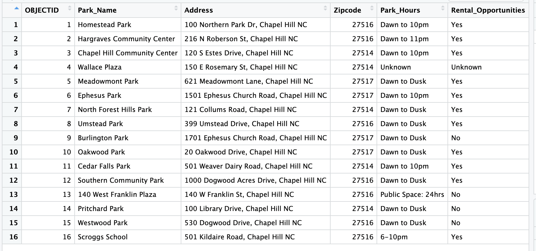
If everything is working, ‘parks’ should appear in your environment. The ‘parks’ dataset is now an “object”.
We can view objects by double clicking the object in the environment. A data table should appear with all the information about the parks.
Add a new code chunk and add the code below to create your first map. Every command that you create should have a comment (#) above that explains what that command is doing. If you run that chunk, a map should appear below.
6.6 Knitting a .Rmd
Knitting a .Rmd means that you create a rendered .html including your code, output, and text. To knit your document, click the knit button. It will create a .html in whatever folder you have the .Rmd saved in (hopefully your GEOG391 folder!)

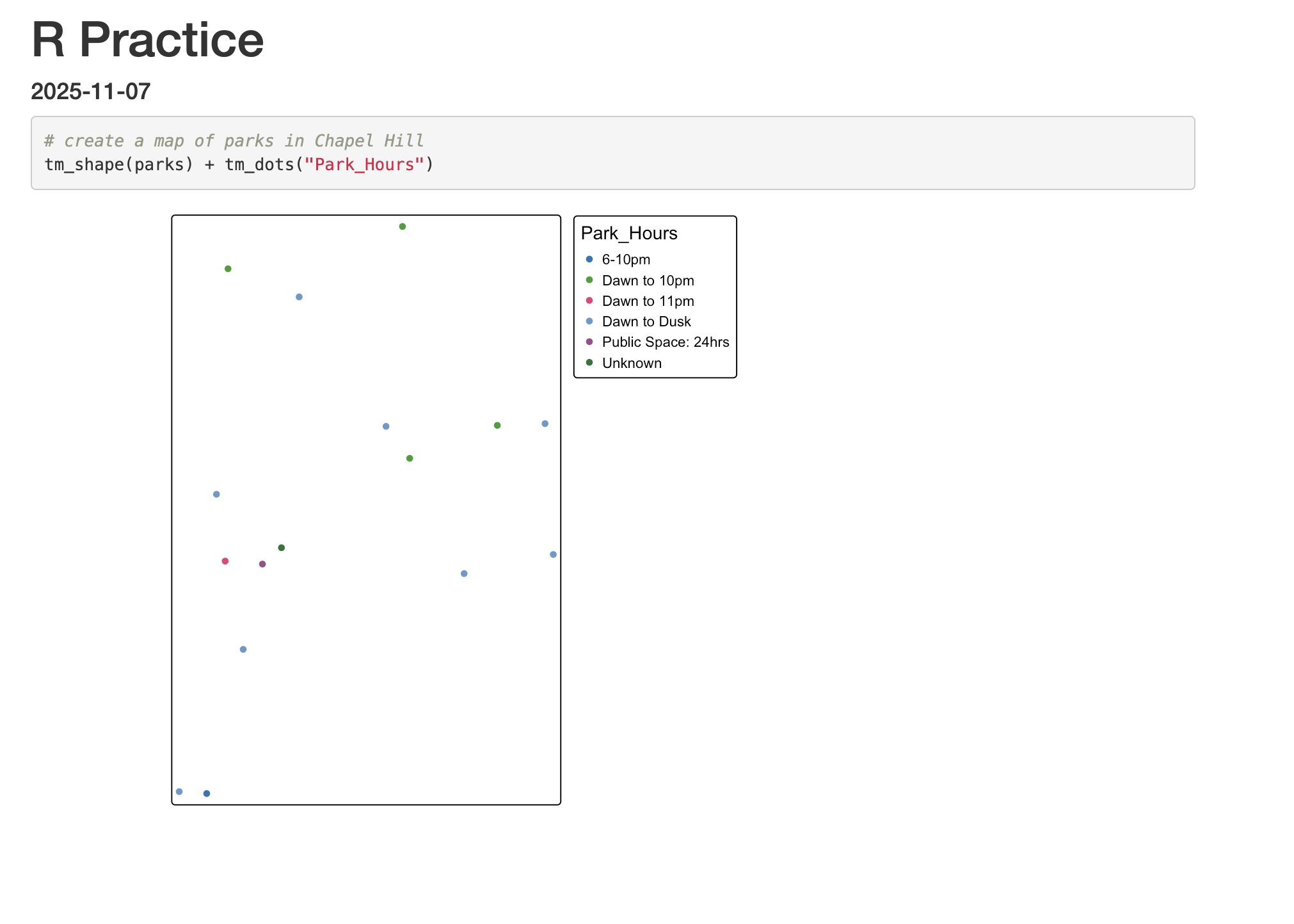
When your knitted document opens, it should look something like this
6.7 Adding Text and Formatting a .Rmd
The great thing about working in .Rmds is that you can create nicely formatted documents that merge code and text. At the bottom of the .Rmd is some tips for formatting nice-looking documents. Play around with adding some heading and text to your document.
Sometimes we want to modify what code and output actually appears in our knitted document. The commands at the bottom of the document explain which chunk modifiers to. See if you can figure out how to change the map chunk to not include the code in the knitted document.
After you are done working in your .Rmd, make sure to save it!