library(tidyverse)
library(tmap)
library(sf)
library(car)

summer_temp <- st_read("https://drive.google.com/uc?export=download&id=1byhsYTBnqegfPGsZWtAHH4pZgGbSTr_s")

acs <- st_read("https://drive.google.com/uc?export=download&id=1ffMbuX4ZQ8vuZK9uwFOBe61bEbKfKg1j") |> mutate(rural = ifelse(rural == 1, "rural", "non-rural"), low_inc = ifelse(low_inc == 1, "low-income", "high-income"), high_commute = ifelse(high_commute == 1, "high commute", "low commute"))

pm <- st_read("https://drive.google.com/uc?export=download&id=1zf1xk-7pOoSnEwGvGsNVa6XejFoPFzdJ") |> mutate(rural = ifelse(rural == 1, "rural", "non-rural"))

mobility <- st_read("https://drive.google.com/uc?export=download&id=1YbCNVR5K8jDF5HOKHcoJ25gz7VkRvDHa") |> mutate(rural = ifelse(rural == 1, "rural", "non-rural"))14 Hypothesis Testing
In this chapter, we will practice common hypothesis testing methods. Hypothesis testing is a statistical approach used to evaluate a claim about a population based on sample data, often comparing differences between groups. This process helps us determine whether observed results are likely due to random chance or reflect a real effect. The p-value of a hypothesis test represents the probability of observing the data (or something more extreme) if the null hypothesis is true. A small p-value suggests that the observed result is unlikely under the null hypothesis.
Most hypothesis tests assume that the sample data is independent, meaning that observations do not have any impact on other observations. Because of the nature of spatial data, we know that this is not true. Because spatial autocorrelation violates the independence assumption of standard hypothesis tests, using these tests can lead to biased test results, underestimated variability, or inflated Type I error rates.
In this chapter, we will practice regular statistical tests, keeping in mind that these tests may not fully account for spatial dependence.
We will use the following spatial datasets:
- A sample of mean summer temperature values across North Carolina from 2000-2010 and 2010-2020 TerraClimate.
- 2023 census tract data from the American Community Survey
- Census tract mean PM2.5 from 2016-2020 from the CDC
- Mobility data during 2020 for North Carolina counties from the Google Covid Mobility Report
To follow along with this tutorial, make a new .Rmd document. As you move through the tutorial add chunks, headers, and relevant text to your document.
14.1 One Sample T-Test
A one-sample t-test is a statistical test used to determine whether the mean of a single sample is significantly different from a known or hypothesized value. It assumes that the data is continuous, that the observations are independent, and the sampling distribution of the mean is normal. While this is guaranteed if the underlying population is normal, the Central Limit Theorem ensures this assumption is met for large samples regardless of the population’s distribution.
To demonstrate a one sample t-test, we can compare the mean daily PM2.5 value for census tracts across North Carolina to a known value. Although each tract in North Carolina has a mean value (i.e. the census tracts are not sampled), we can consider this a “natural sample”.
In geography, inferential statistics are sometimes applied even when datasets include all observed units, because many spatial phenomena contain both systematic and random components. These datasets can be treated as “natural samples”, where the observed variation reflects real-world randomness. For example, mean daily PM2.5 values across all census tracts in a state are influenced by systematic factors like industrial activity and traffic patterns, but also by unpredictable environmental processes such as local weather conditions. This natural variability allows the observed values to be treated as a sample from the broader population of possible PM2.5 conditions, making inferential tests like the one-sample t-test appropriate.
The annual average PM2.5 value for the eastern United States is 7.8µg/m3 . Therefore, we could use a one-sample t-test to see if the North Carolina average differs from the United States average.
Before we run a statistical test, the first thing we have to do is check our assumptions. We know that PM2.5 is a continuous variable. Because this data is spatial, it likely violates the assumption of independence (but we will put a pin in that for now and assume independence) We can estimate the distribution of the population by using the distribution of the sample. A histogram and QQ-Plot indicates that the data distribution is somewhat non-normal.
ggplot(pm, aes(x = meanpm_2016_2020)) + geom_histogram(binwidth = .5)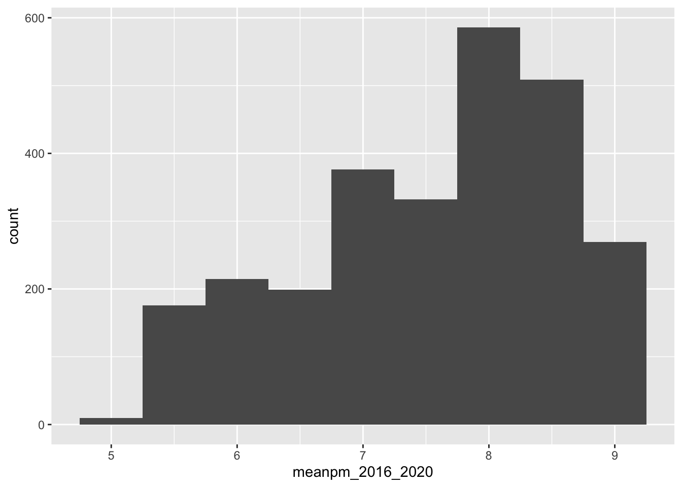
qqnorm(pm$meanpm_2016_2020)
qqline(pm$meanpm_2016_2020, col = "steelblue", lwd = 2)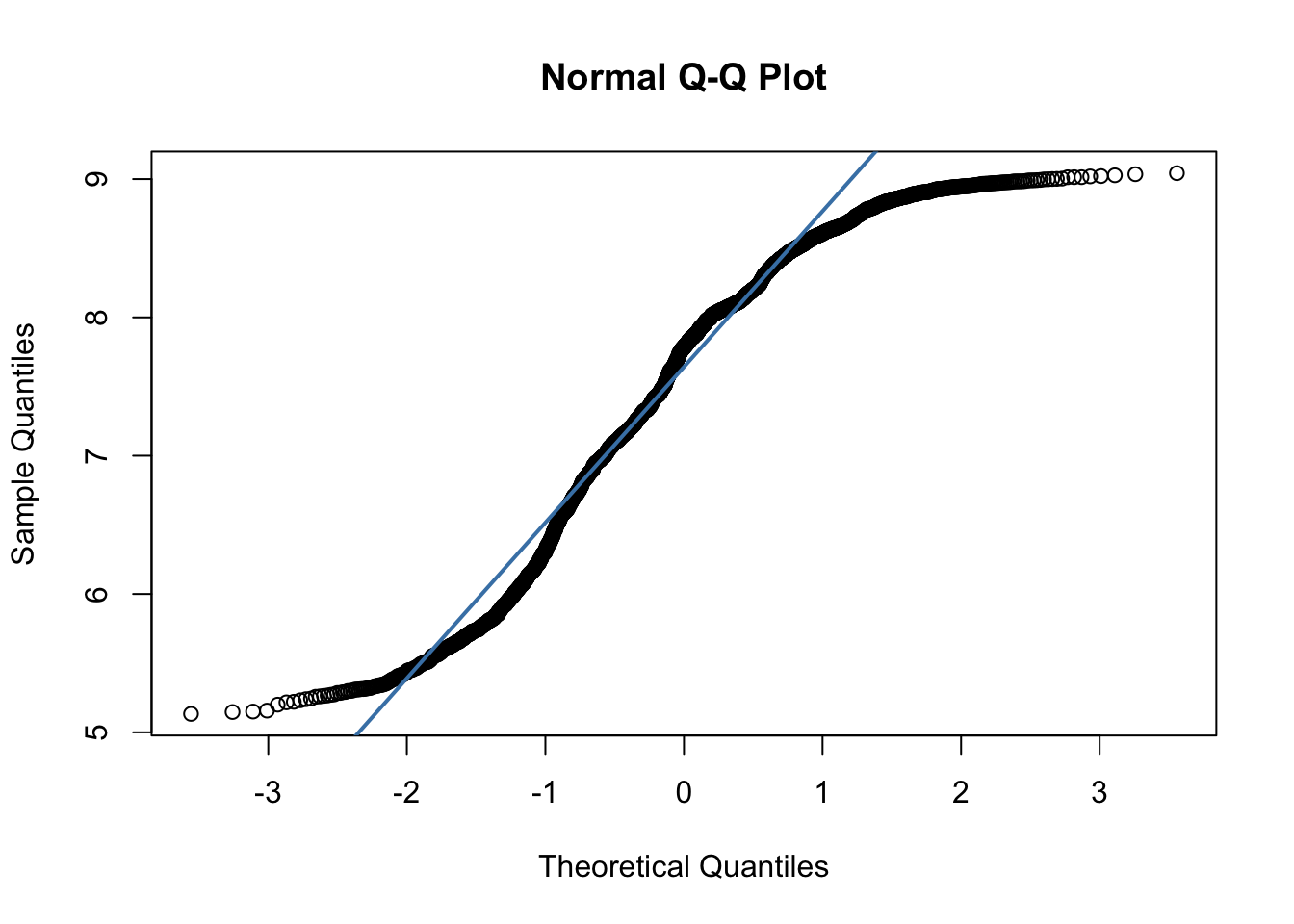
At this point, we have two options for testing whether our sample mean differs from a hypothesized value. The first option is to use a non-parametric test, which does not assume any particular distribution for the population. A non-parametric alternative for a one-sample t-test is the Wilcoxon Signed-Rank Test. The second option is to still use the one-sample t-test. While this test assumes that the population is normally distributed, the Central Limit Theorem tells us that, for large sample sizes (generally greater than 30, but higher for highly non-normal data), the sampling distribution of the mean is approximately normal regardless of the population distribution. Since our sample is large (n = 2672), the t-test is valid in this case, even if the data are not normal.
Since this class focuses on parametric tests, we will continue on with our t-test. The mean of our dataset is
mean(pm$meanpm_2016_2020)[1] 7.546838Q1: Formulate a null hypothesis that would use a one sample, one-sided t-test
We can then test our hypothesis
#test mean
t.test(pm$meanpm_2016_2020, mu = 7.8, alternative = "less", conf.level = 0.95)
    One Sample t-test

data:  pm$meanpm_2016_2020
t = -12.94, df = 2671, p-value < 2.2e-16
alternative hypothesis: true mean is less than 7.8
95 percent confidence interval:
     -Inf 7.579029
sample estimates:
mean of x
 7.546838
In this case, the low p-value of our t.test allows us to reject the null hypothesis in favor of the alternative hypothesis:
H1: The mean PM2.5 value for North Carolina is less than the mean value for the eastern US.
14.2 Two Sample T-Test
A two-sample t-test compares the means of two different samples. For instance, we could compare the mean PM2.5 in urban vs. rural census tracts.
The assumptions for the two sample t-test are the same as the one-sample t-test with one addition: equal variance (also called homoscedasticity). This means that the two groups being compared should have similar variability in their values. If the variances are very different, the standard two-sample t-test may not be appropriate. We can compare the variances a Levene’s test (which is robust to non-normal data)
leveneTest(meanpm_2016_2020 ~ rural, data = pm)Warning in leveneTest.default(y = y, group = group, ...): group coerced to
factor.Levene's Test for Homogeneity of Variance (center = median)
Df F value Pr(>F)
group 1 0.1764 0.6746
2670 In this case, the test indicates no statistical significance, meaning the null hypothesis (no difference in variance) cannot be rejected. If the variances were substantially different, we would need to use a version of the test that does not assume equal variance (Welch’s t-test).
Q2. Formulate a null hypothesis that would use a two sample two-sided t-test.
# Then run a standard two-sample t-test
#if variances were not equal, you would set var.equal = FALSE
t.test(meanpm_2016_2020 ~ rural, data = pm, var.equal = TRUE)
    Two Sample t-test

data:  meanpm_2016_2020 by rural
t = 20.389, df = 2670, p-value < 2.2e-16
alternative hypothesis: true difference in means between group non-rural and group rural is not equal to 0
95 percent confidence interval:
 0.7590222 0.9205533
sample estimates:
mean in group non-rural     mean in group rural
               7.770299                6.930511
Based on our t-test results, we can reject the null hypothesis in favor of the alternative hypothesis:
H1: The mean PM2.5 in urban and rural census tracts is different.
14.3 Paired T-Test
A paired t-test evaluates whether the average change between two paired observations is significantly different from zero. A paired t-test assumes that data is continuous, and the differences between the paired observations are approximately normally distributed. It is typically used when the same individuals or locations are measured at two time points or under two conditions. For instance, we could consider our summer temperature values. In this dataset, we have a sample of 480 locations and two different values– mean summer temperature from 2000-2010 and mean summer temperature from 2010-2020.
We can consider this dataset a true simple random sample.
First, to test the assumption of normally distributed differences, we can examine a Q-QPlot of the differences. Because the paired t-test is robust to moderate non-normality when sample sizes are large, it is still appropriate to proceed with the test.
#add a column with difference
summer_temp <- summer_temp |> mutate(diff = av_summer_2010_2020 - av_summer_2000_2010)

ggplot(summer_temp, aes(x = diff)) + geom_histogram(binwidth = .05)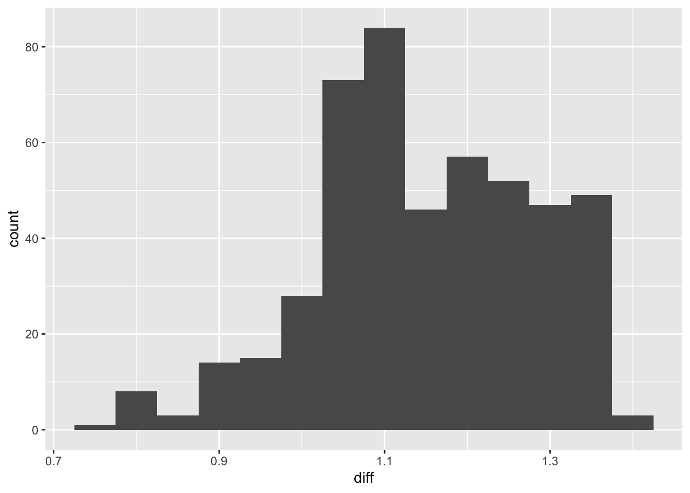
qqnorm(summer_temp$diff)
qqline(summer_temp$diff, col = "steelblue", lwd = 2)
Q3: Formulate a null hypothesis that would use a one-sample paired t-test
t.test(summer_temp$av_summer_2010_2020, summer_temp$av_summer_2000_2010, paired = TRUE, alternative = "greater", conf.level = 0.95)
    Paired t-test

data:  summer_temp$av_summer_2010_2020 and summer_temp$av_summer_2000_2010
t = 192.75, df = 479, p-value < 2.2e-16
alternative hypothesis: true mean difference is greater than 0
95 percent confidence interval:
 1.139164      Inf
sample estimates:
mean difference
       1.148988
Based on our t-test results, we can reject the null hypothesis in favor of the alternative hypothesis:
H1: The mean summer temperature in 2010-2020 is higher than the mean summer temperature in 2000-2010.
14.4 Chi Square Test of Independence
The Chi-square test of independence is a statistical test used to determine whether two categorical variables are associated with one another. Because the variables are categorical rather than continuous, the test is non-parametric, meaning it does not assume any particular underlying distribution. Our American Community Data includes three categorical variables:
- Rural/ Non-rural
- Low income/ High Income
- Low commute / High commute
We could examine whether any pair of these variables is related. For instance, whether rural/non-rural and low commute/ high commute is related. In this case, the null hypothesis would be:
H0: Rural/non-rural status and commute category are independent (there is no association between them).
We can start by looking at a contingency table.
table(acs$rural, acs$high_commute)
            high commute low commute
  non-rural          310        1620
rural 118 580chisq.test(table(acs$rural, acs$high_commute))
    Pearson's Chi-squared test with Yates' continuity correction

data:  table(acs$rural, acs$high_commute)
X-squared = 0.20909, df = 1, p-value = 0.6475
In this case, our X-squared value is low (.209) and the p-value is high (.65), meaning that we fail to reject the null hypothesis.
Q4: Run a chi square test of independence for another set of variables
14.5 Mini Challenge
This challenge will ask you to run hypothesis tests on mobility data for North Carolina counties during Covid-19. We will consider the county values as a natural sample for North Carolina. The mobility dataset includes the following variables:
rural- rural/nonrural flag for each countyworkplace_change- percent change in workplace mobility from March-May 2020workplace_change_may_dec- percent change in workplace mobility by county from May 2020- Dec 2020
- Create two maps– one for each mobility variable. Do you notice any spatial patterns?
- Develop a null hypothesis regarding the relationship between change in workplace mobility between the two time periods. Run a paired t-test between the two time periods to test your hypothesis.
- Develop a null hypothesis regarding the relationship between change in workplace mobility between urban and rural areas (you can pick which workplace change variable to use) . Run an independent samples t-test between the two geographical regions.
- Consider that the known average mobility during the March-May period across the US was -32. Calculate the mean for North Carolina and develop a null hypothesis about the relationship between North Carolina mobility and average US mobility. Run a one sample t-test between the known value and the sample value.