5  Spatial Data Models

When translating real-world features into geographic data, there are two main “conceptual” views of the world: the field view and the object view. A field view treats the world as a continuous surface, where each location is associated with one or more attributes. In contrast, an object view conceptualizes the world as made up of discrete entities that have clearly defined boundaries and exist in specific locations. Between these objects, there can be empty space with no associated features. 

These conceptual models align with two major data models used in GIS. A vector-based model represents geographic features as sets of points, lines, or polygons. This is well-suited for discrete objects. A raster-based model, on the other hand, represents space as a grid of regularly spaced cells, each containing a value that represents an attribute at that location. This structure is ideal for continuous data, where each cell captures a small piece of a surface.

Together, these models allow geographers to choose the most appropriate representation depending on the nature of the phenomenon being studied. The selection of data model then impacts what kinds of spatial questions can be asked about the data, what analysis operations are possible on the data, and how patterns and relationships are interpreted across space. 

5.1 Vector Models

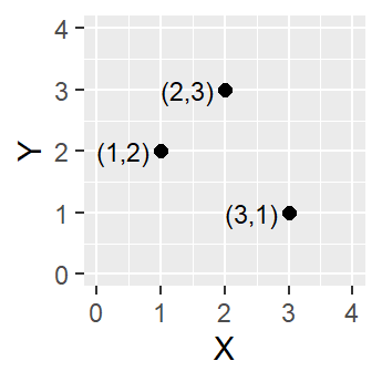
Vector data is built around geometries, which are encoded into the file. The most basic geometry type is a point. A point is represented as a single coordinate pair (x, y).

Points, Intro to GIS and Spatial Analysis, CC BY-NC 4.0

Points, Intro to GIS and Spatial Analysis, CC BY-NC 4.0

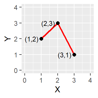
Points can then be combined to create lines and polygons. To create a line, at least two distinct points must be connected

Line, Intro to GIS and Spatial Analysis, CC BY-NC 4.0

Line, Intro to GIS and Spatial Analysis, CC BY-NC 4.0

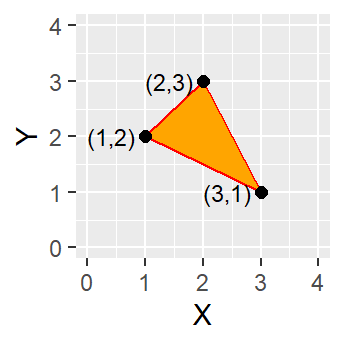
A polygon is created when three or more line segments are connected which means the starting and ending coordinate pairs must be the same. Of the three basic geometric primitives (point, line, polygon), only polygons have an area.

Polygon, Intro to GIS and Spatial Analysis, CC BY-NC 4.0

Polygon, Intro to GIS and Spatial Analysis, CC BY-NC 4.0

5.1.1 Resolution in Vector Data

With vector data, resolution is defined by several conditions: 

  1. The precision of the coordinates
  2. The complexity of the shape (for instance, how many vertices are used to represent the feature)
  3. The minimum mapping unit (MMU). This represents the smallest feature that would be included in the dataset

5.1.2 Topology

Many spatial analysis processes are dependent on topology, which expresses the spatial relationships between connecting or adjacent features. Topology is made up of three separate conditions:

  • Adjacency – which vector features are next to each other? This is essential for tasks like neighborhood analysis or identifying shared boundaries, such as zoning districts or land parcels.
  • Connectivity – which arcs (lines) connect to each other? This underlies network analysis, such as routing or tracing flows, and is determined through arc-node relationships that define from-nodes and to-nodes.
  • Containment – which vector features are within other polygons? This allows GIS to determine spatial inclusion, such as identifying which buildings fall within a flood zone or which parks contain recreational facilities.

Within vector data representations the topological data model explicitly encodes topological relationships. On the other hand, the spaghetti data model does not encode topology. In this model, each feature is stored independently, as a separate set of coordinates, and spatial relationships must be inferred by comparing coordinates. 

While the spaghetti data model is simpler to store, there is a higher risk of topological errors. Topological errors include:

  • Unclosed polygons (boundary does not fully loop)
  • Slivers (small gaps or overlaps between polygons that should be adjacent)
  • Undershoots (two lines that should meet don’t)
  • Overshoots (a line extends beyond the point it should connect to)

These types of errors can seriously impact spatial analysis. Consider a routing analysis where the lines represent street segments. Undershoots and overshoots would restrict driving access on roads that should be accessible. 

QGIS uses on-the-fly topology to build temporary topological relationships for data stored in a spaghetti model. QGIS can also check for potential topology errors and set topology rules (for example, polygons must not intersect).

5.1.3 Common Vector Data File Types

Shapefile (.shp): By far, the most common vector data file type you’ll encounter when accessing geospatial data is the Shapefile (.shp). This format, which is semi-proprietary (structured and maintained by ESRI), has become the dominant standard. This is not because it offers superior functionality, but because of ESRI’s early dominance in the GIS software market. Shapefiles are a non-topological format made up of several files, including the .shp (geometry), .shx (shape index), .dbf (attribute table), .prj (projection), and sometimes others. Despite their ubiquity, shapefiles come with serious limitations: a maximum file size of 2 GB, field names limited to 10 characters, and a maximum of 255 fields. Many believe, myself included, that Shapefile must die!

GeoPackage (.gpkg): GeoPackage is a relatively modern, open-source format developed by the Open Geospatial Consortium (OGC). Built on SQLite, it allows multiple layers and attribute tables to exist within a single .gpkg file, streamlining data management and reducing file clutter. This structure also supports more advanced querying, similar to what’s possible in a relational database– for example, joining attribute tables, filtering by SQL expressions, or performing spatial queries within the file itself. 

GeoJSON (.geojson): GeoJSON is a lightweight, text-based format for encoding vector features using JavaScript Object Notation (JSON). It is especially popular in web mapping environments, where its structure is easily parsed by browsers and APIs. GeoJSON is limited to WGS84 coordinates. 

File Geodatabase (.gdb):The File Geodatabase is a high-capacity, high-performance format developed by ESRI for use with ArcGIS. It stores vector data, rasters, attribute tables, topological rules, subtypes, and more in a structured folder system. This format supports large datasets (into the terabytes), long field names, and complex relationships between layers. While it’s proprietary and not natively supported by all software, it provides powerful data management and analysis capabilities within the ESRI ecosystem. 

5.2 Raster Models

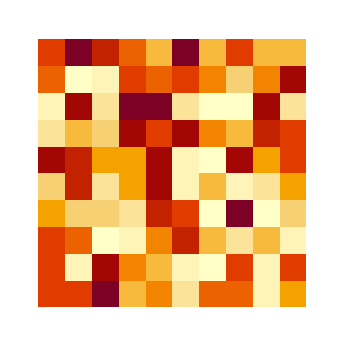
In a raster model, real-life features are represented as an array of pixels. Instead of distinct geometries, a raster is made up of regularly spaced pixels of identical sizes, and each pixel is associated with a value. 

Raster, Intro to GIS and Spatial Analysis, CC BY-NC 4.0

Raster, Intro to GIS and Spatial Analysis, CC BY-NC 4.0

5.2.1 Resolution in Raster Data

In raster data, resolution refers to the size of each pixel, typically expressed in ground units (e.g., feet or meters. ). Smaller pixels mean higher resolution, capturing more detail. Most raster sources, such as satellite imagery, have fixed native resolutions determined by the sensor’s capabilities.

Raster with Multiple Resolutions, Source: National Ecological Observatory Network (NEON)

Raster with Multiple Resolutions, Source: National Ecological Observatory Network (NEON)

5.2.2 Topology in Raster Data

In raster data, topology is implied by the pixel positions, which means that it does not need to be formally encoded. Adjacency can be analyzed by identifying neighboring pixels, connectivity by analyzing whether pixels with the same value form a continuous region, and containment is often analyzed by using a mask defined by a vector data feature. 

5.2.3 Common Raster Data File Types

GeoTIFF (.tif): GeoTIFF is the most widely used raster data format for geospatial applications. It’s a standard TIFF image that includes embedded geographic metadata (like coordinate system, bounds, and resolution), making it easy to georeference. GeoTIFFs are versatile, lossless, and widely supported across GIS platforms. They can store single-band or multi-band imagery, making them suitable for satellite images, elevation data, and classified rasters.

NetCDF (.nc): NetCDF (Network Common Data Form) is a format commonly used for storing multidimensional scientific data, such as climate variables or oceanographic models. It supports time-series rasters, multiple dimensions (e.g., x, y, time, depth), and internal compression. NetCDFs are favored in academic and environmental modeling contexts, but can be complex to manage without specialized tools.

5.3 Selecting a Data Model

In most cases, the type of data being collected or used will determine which data model is most appropriate. Continuous phenomena should be represented as rasters (elevation, climatic variables, etc). Discrete features should be represented with vector models (roads, buildings, property boundaries). Raster data is ideal for surface analysis, remote sensing, and modeling gradual spatial change. It supports powerful cell-by-cell calculations, but can result in large file sizes and less precise feature boundaries. Vector data is more compact and precise, and supports operations like buffering, network analysis, and spatial joins. However, vector files can be more complex to manage when dealing with continuous change or extremely large datasets.

5.4 Coordinate Systems and Projections

To represent the location of features, both data models rely on coordinate systems. Coordinate systems assign a numerical value to each unique location on Earth. When we import spatial data into our GIS, we use these coordinates to make sure that things are located where they should be on the map. There are two main types of coordinate systems that we use in a GIS: geographic coordinate systems (GCS) and projected coordinate systems (PCS). This incredibly informative chapter on Coordinate Systems means that I don’t have to write my own. 

Coordinate systems are defined by whoever produced the data. However, they can be reprojected, or translated to a different coordinate system, depending on your mapping needs. There are common reasons that you would want or need to reproject your data. The common reasons are detailed below:

  1. You are trying to do spatial analysis that relies on distance. If your data is in a GCS, this means that distances are measured in angular degrees, not in a standard distance measurement (like feet, meters, etc.). Angular degrees have different distances depending on how near/far you are from the equator. For example, one degree of longitude is about 111 km at the equator, but much less near the poles. Therefore, for any analysis involving distance, area, or buffering, you should use a projected coordinate system (PCS) with linear units. 
  2. You have data in different coordinate systems. In general, when you are doing analysis across different coordinate systems, you should use a common coordinate system. 
  3. Local accuracy is important. Some projected coordinate systems are designed to minimize distortion in a specific region (e.g., a state plane zone). If you’re doing detailed work in a specific area, using a locally optimized projection will increase accuracy in measurements and reduce spatial errors.
  4. Your analysis would benefit from limited distortion in one (or several) spatial properties. For instance, an analysis of property parcels might need to limit area distortion to ensure that calculated parcel sizes are accurate. In this case, choosing an equal-area projection would help preserve the integrity of area measurements, even if it introduces distortion in shape or distance.

QGIS allows you to reproject, as well as change coordinate systems. These are not the same thing! Reprojecting a layer means actually transforming the data from one coordinate system to another, permanently changing the coordinates stored in the file. This creates a new dataset with new X/Y values based on the target projection. You do this when you want to match coordinate systems across layers or prepare for accurate spatial analysis. Changing the coordinate system in QGIS means telling QGIS how to interpret the coordinates—without changing the data itself. This is sometimes called assigning or defining a projection. You do this when a layer was saved without projection information (or with the wrong one), and you need to clarify what system it’s in.

5.5 Case Studies

5.5.1 Floodplain Management in Chapel Hill

The Town of Chapel Hill is interested in analyzing flood risk to buildings across town. They produce two different interactive maps to present to the town council. Look at the maps below and answer the following questions:

  • These maps both show buildings across town as well as the floodplain (flood risk areas). How do the maps differ?
  • How would these differences impact the outcome of an analysis of building flood risk?

5.5.2 Building Age

The North Carolina Department of Environmental Quality is considering doing outreach for the Energy Saver NC program. They want to target areas in Orange County that may have aging infrastructure and have data on the average year that homes were built in different census enumeration units. Explore the maps below and ask yourself the following questions:

  • These maps both show maximum heat. How do the maps differ?
  • How would these differences impact the outcome of an analysis of average home age?
  • What key geographic concept is this case study displaying?

5.5.3 July Heat Wave

In July 2025 there was a heat wave across the southeast US. A nonprofit group that is focused on planting trees in areas impacted by the urban heat island affect is given two raster datasets that display maximum land surface temperature (LST) on the hottest day of the heatwave. The nonprofit plans to use this data to identify specific streets across Orange County where more trees should be planted. Explore the maps below and ask yourself the following questions

  • These maps both show maximum heat. How do the maps differ?
  • How would these differences impact the outcome of an analysis identifying tree planting priority areas?